Philipp Dapprich Interview on Democratic Central Planning Part 2 – Simulations, Opportunity Cost, Environment, Multiple Techniques, Computation

mέta & After the Oligarchy

Editor’s note: Discussion includes using choice of production technique in central planning, opportunity cost, labour cost, calculating environmental costs (such as GHG emissions), agent-based modelling, consumer modelling, simulation results, computational complexity, research to be done.

[After The Oligarchy] Hello fellow democrats, futurists, and problem solvers, this is After The Oligarchy. Today I’m speaking with Dr. Philipp Dapprich.

Philipp Dapprich is a political economist and philosopher working at the Free University Berlin. His PhD was entitled Rationality and Distribution in the Socialist Economy (2020), , and he is also co-author of a forthcoming (2022) book entitled Economic Planning in an Age of Environmental Crisis. Today we’ll be discussing his work on refining the model of economic planning first proposed by Cockshott and Cottrell in Towards a New Socialism (1993).

Today’s conversation is in association with mέta: the Centre for Postcapitalist Civilisation if you’re not familiar with Towards a New Socialism you can buy the book or find a free PDF online you can also find interviews with Paul Cockshott on this channel and I’ll put links in the description to Philipp Dapprich’s doctoral thesis as well as a relevant paper.

Philipp Dapprich, thank you very much for joining me.

[Philipp Dapprich] Thank you for having me again.

[ATO] The first thing I’m going to say is I really recommend the viewers watch the previous interview, because they’re not standalone interviews. We covered a lot of important stuff last time about opportunity costs, the motivations for your work, and really if viewers want to understand what we’re talking about now they should watch that. So, I’m just going to say that once.

Today there are two main things that we want to talk about. The first is we want to get into the details of the simulations that you ran to investigate your new techniques of opportunity cost valuations in the Towards a New Socialism model.

The other thing is we want to talk about a fundamental question, a fundamental problem, in economic planning and central planning about choice of production technologies. Can you introduce the problem and how you approached it?

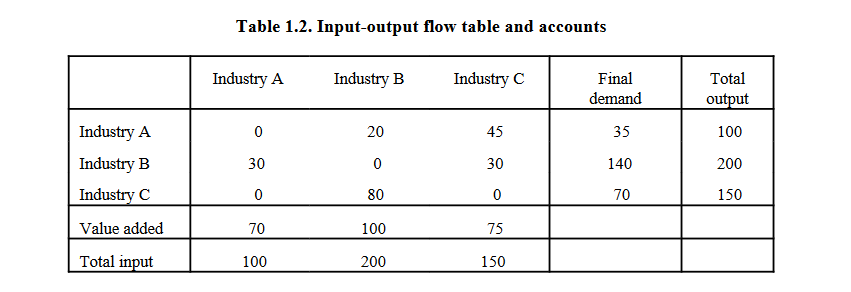
[PD] One approach to planning has long been to use so-called input-output tables. And input-output tables – they are commonly published even by western capitalist countries – show you which industries use inputs from which other industries, and which output, how much output, they produce with this.

And the problem with that is that these tables are generally very aggregated. So, you have entire industries, you might have something like Forestry and Agriculture, all bunched together into one column of the table. And it doesn’t differentiate between various different kinds of products within those industries. It won’t differentiate between different kinds of agricultural products, lumber, and so on. That’s the first problem: they’re way too aggregated. And what you’d have to do is to have a much more disaggregated table which differentiates between different kinds of products.

[ATO] When you’re talking about input-output tables – for viewers – you’re saying that these are very aggregated tables. And they’re saying, for example, the agricultural sector is outputting let’s say corn and milk. And then you’re also looking at the inputs required for that, for example, grain, iron, electricity.

[PD] Exactly. The input-output table will tell you not just how much the Forestry and Agriculture sector is producing, but also which inputs from which other industries it is using. Is it using a lot of input from the energy industry, or from the mining industry? How much labour is it using? That’s an important input as well.

But, as I said, it doesn’t differentiate between different kinds of products being produced in those industries. It’s all aggregated into one column. And if you want to plan specifically, not just what the size of a certain sector should be, but precisely which kinds of products should be produced – and that’s the level of detail of planning that we really need – those input-output tables are not going to be very useful.

So, the first thing you have to do is get a much more disaggregated table which differentiates within the same industry between different kinds of product. For example, you differentiate between wheat, potatoes, and tomatoes, and so on, rather than having them all bunched together as one sector. That’s the first problem, that they don’t differentiate between different kinds of products.

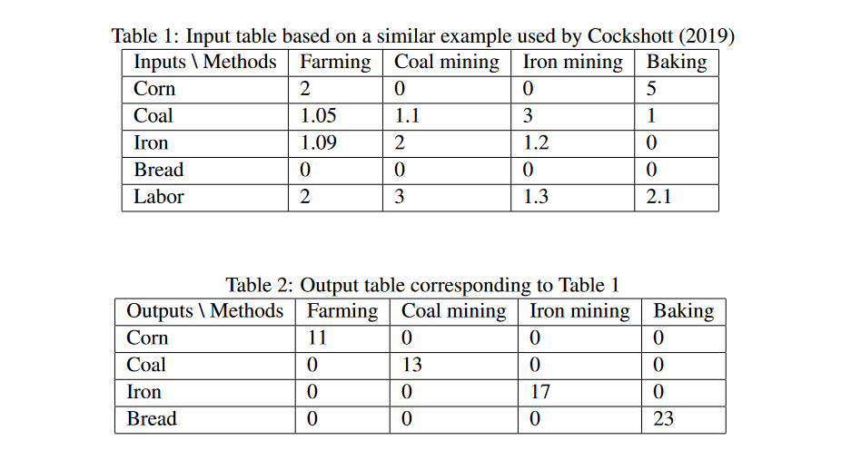
The second problem is they don’t differentiate between different ways of producing that product. The input-output table looks at the past year, or whatever year this table was made for, and looks at how much was used in this industry to produce whatever that industry produces. So even if we were to differentiate that, and we look at potato farming or we look at electricity generation (maybe that’s a better example here) it will not differentiate between electricity that’s produced by coal power plants versus nuclear power plants, versus solar and wind power plants. But if you want to plan precisely which methods should be used, you need to be able to differentiate this. Instead, an input-output table just tells you at the current mix of electricity production this is how many tons of coal were used to produce electricity, this is how many wind turbines were installed, and so on, this is how much labour was being used in in the electricity industry.

So, you don’t just want to differentiate between different kinds of products. Here we’re talking about the same product, electricity, but there are different methods of producing it. And one of the fundamental questions if you want to determine an efficient allocation of resources is which of these methods should we be using? We have to be able to tell them apart.

And the way that I do that is I kind of move away from these traditional input-output tables, and instead have tables which don’t have an entire sector or even single product as one column, but instead have a production technique. And producing electricity with coal power would be a different production technique hfrom producing it with wind power or nuclear power, and so on. And each column would then list with this particular kind of production technique how much labour is needed, how much coal would be needed, how many wind engines would be needed, to produce a certain output of electricity. And this can then serve as a basis for determining a production plan which precisely specifies which techniques should be used to what extent to produce the optimal overall output.

[ATO] Thank you for that overview. And let me ask: in a traditional input-output table, like you’re saying, it’s effectively a snapshot of the production techniques which are currently in use. However, if we wanted to devise plan for the economy that was the most efficient, we would of course not only want to find the best distribution of resources given fixed production techniques, but we’d also want to pick what the best production technique for each good and service would be.

So, you’re saying that part of how you approach this is that rather than using a traditional input-output table, you’re now introducing or including separate production techniques into some kind of table or matrix. Like you said, you could have multiple entries for electricity: Electricity 1, Electricity 2, Electricity 3, 4, 5, 6, 7, 8, 9, 10.

Could you talk more about how a planning algorithm can actually choose between these different techniques? Choose between one method of electricity generation over another.

[PD] What I call a plan, in the end, is basically a specification of which production techniques should be used at which intensity. Intensity here means if you use it at an intensity of one, then you’ll have exactly the input stated in the table and the outputs stated in the table. If you use it as an at an intensity of two, that means you’re using it twice as much. Which means you have twice as many inputs, twice as many outputs.

So, a plan in the end is supposed to specify which of these techniques should be used at what intensity. And the idea is that you calculate the plan which uses the mix of techniques which maximizes the overall production output, and that can be calculated using linear programming. So, you can determine the optimal plan, i.e. the mix of production techniques which maximizes overall production.

[ATO] In order for this to function then, presumably, let’s say in the real world, there would have to be some kind of register or list of available production techniques. How could we imagine that operating?

[PD] If you want to imagine some kind of central planning agency being in charge of this planning process in some sense, or administrating it, they would need to have this table which lists all the available production techniques, or at least the ones which plausibly could be used in an optimal plan. They need to have all the entries so they need to know which resources are being used, and which output is being produced by that plan.

The way that I imagine that this table would be created is you could have various production units communicating what production techniques they have available. Or you could also have research centres which continue to come up with new methods and which would then, perhaps in an experimental fashion, determine the resource usage of those production techniques, how much can be produced with those resources using that technique, and then communicate that to a central computer system where this would then be entered into the table.

[ATO] I’m thinking about computation here. And, of course, probably the great attraction of using these Leontief style input-output tables is that they make computation of a comprehensive plan so much easier. Now, if you introduce multiple production techniques, multiple production vectors for each product, that’s obviously going to make it more computationally complex. So, what are your thoughts about this? Is it still feasible and if so, how would you quantify that?

[PD] I think actually the biggest increase in computational complexity comes from differentiating between different kinds of products within the same industry. A typical input-output table will have maybe 100, at maximum maybe 500, different industries but there might be hundreds of millions of different kinds of products. That will massively increase the size of the table and that’s the computational complexity of the problem that has to be solved.

The different kinds of production techniques – if we maybe imagine that there might be two or three, on average, different ways of producing a product, that will of course increase it further. But that’s probably not the most relevant factor here. The differentiation between different kinds of products within the same industry will probably – at least that’s my guess – be the big effect.

The answer is yes absolutely that increases the computational complexity and increases the length of time that a computer will need to solve these kinds of problems

[ATO] Yes certainly, disaggregating the products has an enormous effect and that’s very relevant. I’m asking particularly about different production techniques because I think Cockshott and Cottrell have very convincingly argued that without multiple production techniques a comprehensive plan can be feasibly calculated for on the order of 100 million or a billion distinct products.

What you’re saying is that if we have, say, a handful of leading candidates for production techniques because it’s not necessary to list every single production technique available, including all of the ones which are really inefficient. There is probably a handful of ones which are more or less equally successful, maybe one is better in one aspect, another is better another aspect. You’re saying that, let’s say, if these additional production techniques are on the order of 10 or less, then you’re just looking at multiplying the calculations by a factor of 10.

[PD] Exactly. I think potentially imaginable production techniques can be already excluded from an engineering standpoint, because we already know that they used a lot of certain resources. We could in theory produce electricity by having hamsters on treadmills or something like that, but we know that’s not going to be an economically viable and feasible way of producing electricity compared to nuclear power or wind power or something like that. So, I think a lot a lot can be excluded already.

I actually think there’s a way also to formally calculate that without already having to do the optimization. Which is: if based on past plans, for example, you were able to calculate the opportunity costs of not just various products but also of inputs for these products – we talked about opportunity costs in the last part – if you were to calculate that opportunity cost, you could also use that as a cost indicator to give you a vague idea of the costs of different inputs. And then if you notice this production technique uses a lot of this really valuable scarce resource, that has a very high opportunity cost, that we really need somewhere, else then you can maybe already preclude that from the list to begin with. And that’s not going to be something that would be used in an optimal plan anyway.

[ATO] You’re saying that the opportunity cost valuations could be used to screen for efficient production techniques.

[PD] Exactly.

[ATO] Okay and actually on that point, firstly I’m just trying to picture the introduction of these multiple production techniques for each product. Is that essentially functioning like rather than, say, having electricity as an entry it’s almost like you have now multiple products. We know that they are electricity, but in mathematical terms it’s like there are different products.

[PD] Well, you need a way to specify to the algorithm, to the computer, that these are the same product. Because this will be relevant when calculating which techniques should be used, and how much do we need of a certain product, and so on. So, the algorithm needs to know which product is being produced.

The way I do this is by having actually two different kinds of tables. The first table specifies only the inputs of various production techniques. And then the second table specifies to you which product is being produced with this technique.

One advantage of this is also that you can actually have multiple products of the same production technique. In some production processes you might have maybe the main product but you also have some by-product that is being used. For example, something that has been in the news lately because of high energy prices, fertilizer manufacturers lowered their production but because a by-product of the fertilizer production process is CO2, that is then used for fizzy drinks and other kinds of things, that also reduced the availability of CO2. So, by having these two different tables – one specifies the inputs, the other the outputs – you can then also have in the output table non-zero entries for multiple products. You could have production techniques which produce more than one output.

[ATO] Yes, that’s a good point because that is certainly relevant information for actually quite a lot of products. And if we want to have a more circular economy that’s important information, we don’t want to just throw away products. We want to use by-products as efficiently as possible.

Staying on the topic of computational complexity just for a little bit longer: the opportunity cost valuations, what are the ramifications there on computation?

[PD] The way that I calculated them in my thesis was basically I did one optimization – we talked last time about this free bread method, for example, which might be used to produce one free unit of bread and then you see how that increases the overall output – so you do one calculation without any of these methods and then you do an extra calculation for each product. Basically, to see how much you increase the optimized production output when you have one unit of it for free.

And that, of course, means that you have to do a lot of extra calculations. But there is actually a computationally much easier way of doing this with linear programming. In linear programming, you actually get certain factors which are used in the optimization process which seem to be equivalent to my way of calculating it, and you get these basically computationally for free. So, there isn’t any significant increase in the computational complexity if you also want to calculate these opportunity costs.

[ATO] What you’re saying is that you can actually change from labour time calculations to opportunity cost calculations, which on the face of it would seem to require a lot more computation, but actually at the end of it these two methods – labour cost and opportunity cost – end up with roughly the same order of computational complexity.

[PD] Yes. At least that’s the case if you use linear programming.

The problem is that linear programming still seems to be a bit too complex for the number of different products and production techniques that that we have to consider. But there are better ways of doing that. Cockshott and Cottrell proposed the harmony algorithm – I think Cockshott was actually the one that that developed this – which is more computationally efficient than linear programming in these kinds of planning problems.

What I don’t know is whether there’s also a way of using the harmony algorithm to get these opportunity cost factors. I think that’s something that still needs to be looked into. Whether in the end you can also get these for free using an optimization method which is sufficiently computationally efficient to calculate a plan for millions, hundreds of millions, of different products and production techniques within a time frame that’s acceptable.

[ATO] You’re saying that the opportunity cost valuations actually do add in significantly more computation, so this is a topic for future research.

[PD] Well, they don’t add anything if you use linear programming. But the question is whether linear programming is actually fast enough to solve these kinds of problems. And Paul Cockshott suggests that actually with linear programming it would still require too much time, too much computer time, to solve these kinds of problems. And you actually need a more efficient algorithm and he proposes the harmony algorithm, which does solve it in time.

So, the question is whether what’s true for linear programming – that you can basically get these evaluations for free – is also true for the harmony algorithm. And that’s something that I simply don’t know.

[ATO] This is something to be to be worked out, it’s an open question.

[PD] Yes.

[ATO] All right. Would you be interested in talking about the opportunity cost of land in particular?

[PD] Yes, I mean it’s not that different from other factors really. But we could briefly talk about that.

[ATO] It’s basically the same process?

[PD] Yes, the idea would be that you consider if we had one unit of land extra how much does that increase production.

[ATO] Okay, let’s park that for now because that requires us to go back through all of the material from last interview again.

[PD] Yeah.

[ATO] Last time we discussed in depth the method that you’ve introduced to calculate the opportunity cost of different resources, different goods and services, in a democratic central plan. But also you did some simulations to investigate this, and we didn’t really talk about that much. Would you like to talk about that now?

[PD] Yes, sure, do you want me to just briefly outline it?

[ATO] Yes, please.

[PD] The basic idea of the simulation, or the motivation behind it, is I wanted to see how the composition of products that is being produced will differ in the traditional labour value model and my model using opportunity cost. And, specifically, I was interested in seeing how emission rights – if you constrain the allowable emissions for the economy overall, you put a cap on emissions – affect which kinds of products are being produced.

And I thought the best way of testing that would be a computer simulation. The computer simulation, on the one hand, uses precisely – or at least a simplified version of – the kinds of planning algorithms that you would apply in in the real world.

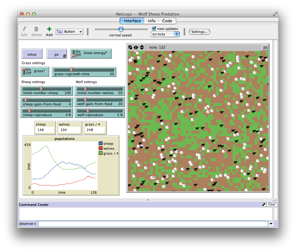
And then, on the other hand, you need to also consider the behaviour of consumers. Of course, in a computer simulation you don’t have real consumers, and in the real world you would, these would be real people going to the supermarket deciding what to use their vouchers, or tokens, or money, or whatever you want to call it, on. But for the purpose of the computer simulation, I devised a very simple agent-based model which simulates the behaviour of individual consumers. And then you can observe with consumers behaving in in this way how would the planning algorithm react to that? How would it change the composition of products that are being produced?

[ATO] Can we just take a brief detour here which I think people might find interesting. Some people will know what agent-based modelling is but others won’t. And I just think it would be interesting if you just explained briefly what that was. Because it’s a different kind of modelling than has traditionally been done for decades and decades, and it’s something that’s become a lot more popular now particularly in economics.

[PD] With agent-based modelling you’re basically modelling individual agents. You’re saying okay well we have maybe a thousand different agents and we’re going to model for each one of them how are they going to behave in a certain situation. How they’re going to act, interact with each other, with the environment, and so on. Which choices, which decisions, are they going to make?

And, of course, then you have some things about how people will react to various circumstances. And there might also be an element of chance. My model does include an element of chance as well, but with probabilities of various decisions depending on certain circumstances and also certain factors you can pre-specify as someone running this simulation.

[ATO] So people can picture this who aren’t familiar with it. You could imagine, for example, if you’re one of these evil ‘security’ corporations trying to prepare the oligarchy to deal with the various uprisings which are due to happen in the in the coming century. You can imagine a crowd control simulation where you have individual people. And you can imagine looking at them, and then there are simple rules which govern their behaviour. Like if they’re enclosed by a certain number of other agents, they might act like this, and so forth.

And so, you program in these very basic rules for what they’re going to do, and then you just watch what happens when you throw all of these marbles together basically, and they interact with each other. And sometimes very surprising things can happen.

Well, anyway that’s agent-based modelling, but you were talking about using that to model consumers in the simulation. So, please continue.

[PD] In my simulation, the basic idea or what I wanted from the consumers is I wanted their decisions to be price dependent.

Basically, what that means is that if the price of a good increases suddenly they should be less likely to buy this kind of product, and maybe choose some alternative instead. Because I wanted to keep it very simple, it is price dependent so you get exactly this result under very specific circumstances. But as long as these are met, then you get significant price reaction of consumers so that they’re less likely to buy a product if the price of that product increases.

But some still will buy it. Some people will still buy a product even if it’s ridiculously expensive. And the real world equivalent would be someone who values this product so much that they’re willing to pay even a very high price for it. And you get some people like that, and you get that in the simulation as well.

The way that I’ve done this is basically each consumer has an infinite shopping list, and the shopping list is ordered. It is procedurally generated; you generate as much as you need basically until the consumer stops shopping. You start off with the first item on the list and that’s the top priority for that consumer. And if the consumer can afford that item, then she or he will purchase that item, and then goes moves on to the second item. And this then continues until the consumer isn’t able to afford an item

I think three times in a row is what I picked here as the stop condition. So, if there are three items on the list in a row that the consumer can no longer afford, because she or he has already spent all of her credits on the items further up on the list, then she’ll conclude that she has run out of money. She can’t afford anything else. He’s going to go home now.

The reason that under certain circumstances this yields a price dependent behaviour -consumption behaviour – is that if the price of a product is more expensive, it is more likely that she will not have enough credits left to be able to purchase that, and she will have to skip the item and see if there’s something else further down on the list that she can still afford.

So, that’s how you get this price dependent reaction with people being less likely to purchase items as their price increases

[ATO] The aim there is you’re trying to create a model of consumer behaviour where consumers are responsive to prices. Because the essential point of this is to model consumer feedback so that they’re responsive to prices. And then you’re saying, also, that this is done in a statistical way. Essentially, there’s a statistical distribution of preferences – that’s what it amounts to. Even if something is very expensive, e.g. there’s a very expensive guitar, somebody will want to buy that. Most people won’t.

[PD] Exactly. Some people will still purchase this.

And also what you get with this agent-based model which you wouldn’t get with – or which would be more difficult to get with – standard neoclassical models, is that the choice of products doesn’t just depend on the price of an individual product. So, how many, say, potatoes we bought doesn’t just depend on the price of potatoes but it also depends on the price of other products. Because if potatoes have a fair price but something else is a real bargain, then people might choose to use their limited funds not to buy potatoes and buy something else instead. That is actually something else that I wanted to capture in this model, and which I’ve accomplished, that the amount of a product being bought doesn’t just depend on its own price but also on the price of everything else that could be bought instead.

So, these are the two important factors that I cared about and which are realized in the model.

But, of course, overall it’s not a particularly realistic model of how people behave. It’s not supposed to be. If you were to apply this model in the real world, you wouldn’t need this consumer model in the first place. You’d have real people doing this. So, realism is not necessarily what I was interested in. These two factors are what I care about: price dependent behaviour of consumers, and that the amount of the product being bought doesn’t just depend on its own price but also on the price of alternative products.

[ATO] You’ve got that consumer model, but of course your overarching goal isn’t to model consumer behaviour. That is in the service of a larger goal which is an optimal plan. So, let’s talk about the other aspects of the simulation.

[PD] The way these two parts then fit together – you have, on the one hand, this optimal planning algorithm, the consumer feedback mechanism which we talked about last time, and the consumer behaviour model. The consumer model tells you what the consumer feedback going to be.

So, at a given supply … The optimal plan tells you how much is being produced of various products, that tells you how much is available for consumers. That’s the supply that can then be compared to the demand at a certain price level. You market the consumer products at certain prices to consumers, and you see what is going to be the demand for various products based on the consumer model.

Then you have supply and demand, and you can compare these. And you might observe that actually at the current prices the demand for a product is really high higher than the supply. And then based on one of these two feedback mechanisms – which we talked about last time – you’d adjust the price to try to balance supply and demand.

So, in this case, you would increase the price, and because the consumer model is reactive to these prices that means demand will go down. If the opposite is the case, so actually at current prices the demand for product is much lower than what’s been made available through production, than the supply, then you actually lower the price to encourage more consumers to pick these kinds of products, so that they don’t go to waste.

That’s the first step, this comparison of supply and demand. And this is really where the consumer model interacts with the planning algorithm and the feedback methods that we talked about last time.

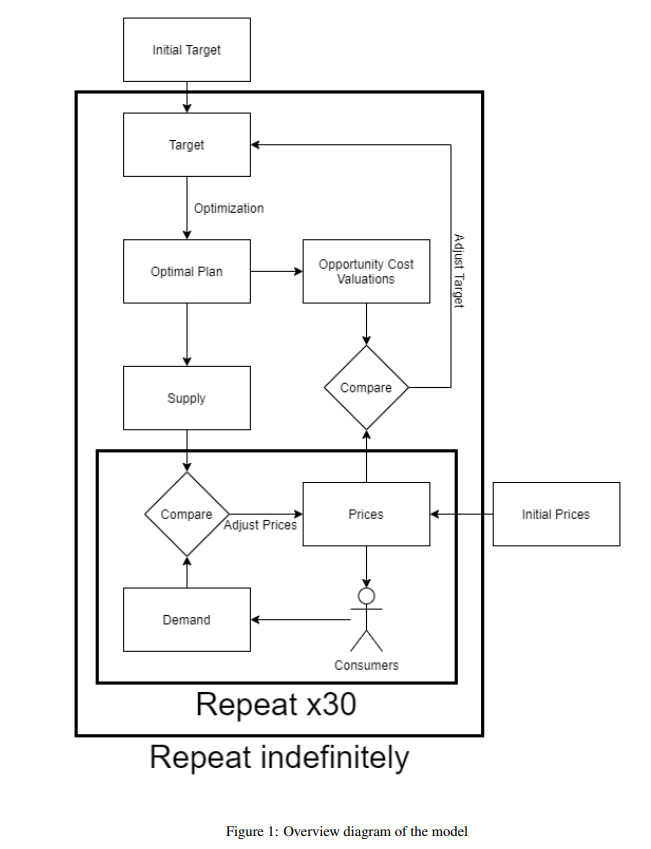
This is then done 30 times. You can imagine that that this is one month consisting of 30 days, and every day we adjust the prices somewhat to try to create this match of supply and demand. What I found in the very simple simulations that I ran is that usually after around 20 days you’d have a pretty good match of supply and demand. It took 30 [days] because I also thought that fits well with one month, so we can maybe better imagine that. After this 30 day period, usually you’ll have the market clearing prices which match supply and demand.

Now you know what the market clearing prices for a product are. You can also calculate the opportunity cost, in the way that we discussed in the last interview.

And now you have to make them comparable. The way that you do it is you now have the market clearing prices after this 30-day period, and you can also calculate the opportunity costs in the way that we discussed the last time for various products. You now have to make these two comparable because they might be on completely different scales. You want to (what’s called) ‘normalize’ them, bring them on the same level.

And the way that I do that is I modify the opportunity costs such that the relative costs of various products remain the same. So, originally, one item costs twice as much as another item. Those relations will be maintained. But the overall cost of all the different products that have been produced will be the same now, after normalization, as the overall price at the market clearing prices of all the products that are available. You maintain the proportions of different costs while having them on the same scale as market clearing prices, so that market clearing prices and opportunity costs of products can now be compared.

[ATO] Just to make that concrete for viewers: so, you’ve calculated that the opportunity cost of bread is – I’m just going to pick random numbers – a thousand euro, or a thousand, let’s say. And for potatoes the opportunity cost is 500 euro. If you look in the shop, then price of bread is one euro and the price of potatoes is 50 euro. So, first of all you’re saying that the proportions are the same, the relative prices, are the same. But you can’t compare an opportunity cost of bread which is a thousand euro with the price of bread which is one euro. That’ll end up with nonsense.

[PD] Well, the proportions won’t necessarily be the same with opportunity costs and prices. The opportunity cost of producing one unit of bread might be twice as much as producing one unit of potatoes. But the price of it actually might be three times more. So, that can still be the case.

But what you want to avoid is that they are on completely different scales. You assumed opportunity cost is already measured in euro, or something like that. Now the opportunity cost is not being measured in the same unit as the credits, or the vouchers, or the or the money, that you’re using to purchase items at all. They’re not measured in the same unit.

So, you have to make them comparable in some sense. And, as I said, the way doing it is not to change the proportions of the cost. That would stay two to one, even if the price is three to one. You maintain these proportions. But the overall value of all the products has to perhaps be reduced. Let’s say, on average, the cost of producing an individual product is a thousand but the price of it on average is one. Then you have to reduce the cost by a factor of 1,000, reduce that for all products to make them comparable. That’s the basic idea.

[ATO] While prices would be recorded in some units – we could imagine it might be something like euro – the opportunity cost valuations, that measurement is in terms of fulfilment of the plan. It’s a fulfilment of the target vector, so it’s not it doesn’t have the same unit as a price.

[PD] Yes, the unit is whatever the unit of the objective function is, which could be tons of grain for example. Because you see a slight increase in the value of the optimized objective function, and that’s what you’re measuring here: the opportunity cost.

But you then want to make that comparable to prices. So, you might have to scale the opportunity costs down a bit, or scale them up, while maintaining their proportions. You might increase them by a factor of a thousand, or decrease them by a factor of a thousand, something like that, such that in the end the overall cost of all items available is the same as the overall price of all items available.

[ATO] So, what’s the next step?

[PD] The next step is now, after this 30 day period, you have the market clearing prices for items. You can also calculate the opportunity cost for the items. You scale the opportunity costs to be comparable to the prices, and then you compare them.

So, for each product you would look: well, the price for that item is maybe 10. But the cost of producing it is only 9. And then, because the price is higher than the cost, it means there’s a lot of demand even at a high price for this product, which means we should be producing more of this. People are willing to pay the cost of producing this item. And actually there are even people are willing to pay more than that. So, we’ll produce more of it in the future.

And so you adjust the plan target entry for that product. The plan target, to repeat from last time, specifies the proportions in which various products are being produced. If our example is bread, and you have a price for bread that’s higher than the opportunity cost, and then you increase the entry for bread such that in the next planned period, we’ll have a higher proportion of bread being produced in the output mix.

If the opposite is the case, let’s say for potatoes, the market clearing price is actually lower than the opportunity cost of producing potatoes, then you decrease the entry for potatoes in the plan target vector (which specifies the proportions at which things have been produced). And what you then get is basically in the next planned period – a few days, the next month – you’d be producing relatively more grain compared to potatoes. Because you’ve now increased the proportion for grain and decreased the proportion for potatoes. So, you have the higher emphasis on bread versus potatoes.

[ATO] You’re talking about using the comparison between the opportunity cost of a product – let’s say, bread – with the price that it’s selling for. Those are being compared, and then the plan target is being adjusted based on that comparison. If the price is higher than the opportunity cost, this is taken as a signal that it would make sense for more of this to be produced. Because people are willing to pay more than the calculated cost of producing it, which is the opportunity cost.

And similarly in the reverse case. If the opportunity cost is higher than the price, people aren’t actually willing to pay a price which is equal to the opportunity cost. Then that’s an indication that too much of it is being produced.

And so, the plan target, which is basically a recipe for the entire economy – we talked about that last time, the example was falafel. If you want to make falafel, then you have one tin of chickpeas, one portion of garlic and two of parsley. But this is for the whole economy.

[PD] Let me just correct you there. The plan target is not what you might call a recipe. It doesn’t tell you what you need to produce falafel. Rather, it tells you how much falafel should you produce relative to haloumi, and kebab, and other things. Because if you produce too much falafel, there actually might not be that many people who want to eat falafel. Maybe more people want to eat haloumi instead. So the plan target tells you the proportions in which various products should be produced.

A different table, the input table, would tell you what you need to produce it. that that would be the recipe, or the plan target tells you how much of various things to produce in proportion to other things.

[ATO] That’s completely true. And when I was saying that, I was thinking, well, this is actually a very confusing analogy, because the natural analogy of falafel will be an actual would be an actual product in the economy, whereas I’m talking about in the economy, What I was trying to get across when we went through this last time, was that if you’re producing one unit of potatoes, then there will also be produced two units of iron, five units of bicycles, three units of electricity. And, like you said, they’re fixed proportions. So that’s where I was going with the recipe – that it scales up in fixed proportions.

The point being that comparing the opportunity cost to the price – this feeds back then and changes that plan target. So, the proportions will change. If people don’t want bread, then the amount of bread in this plan target will decrease.

Okay, so now know what?

[PD] Yes, exactly. So, now you change the plan target. You change the proportions at which various consumer products are being produced. Basically the idea is to adjust them to what people actually want and need. And then you have a new plan target. And based on that, you can then calculate a new production plan for the next period.

So you had some initial plan target that you started off with. You’re now changing that plan target, somewhat adjusting that in response to the behaviour of consumers. And now you start in the next period and you do the same thing basically again. So, you’ll have a slightly different composition of products now. You’ll again market them to consumers, every day you adjust the price until you approach market clearing prices. And then at the end of the period, again the same for the third period, you would adjust the target and recalculate the plan.

So each plan period you get a slightly different composition, and it keeps being adjusted to match what consumers actually are willing to spend that vouchers or credits on.

[ATO] The way you’ve done this is that the consumer model runs for 30 iterations, which we could think of as 30 days, or a month, consumers going into shops and buying things and liking the prices, or not liking the prices, and changing their demand. But if we just think about the real world, would you envisage this model applying in real life in a similar way? That the plan target might be updated once a month? Or is this just the way the simulation functions?

[PD] This is just the way I did it in the simulation. How are you going to do it in the real world depends, for example, on how long it takes to calculate an optimal plan. So, if it only takes a couple of minutes, then maybe you can update it every day. If it takes a couple of days, then maybe once a week, or once a month is more realistic.

But I needed to choose some number here. And also the other factor was I wanted for the simulation at least sufficient time for prices to adjust to market clearing prices before I calculate a new plan. That’s why it shows this 30 day period.

In the real world, of course, you could adjust it depending on how fast prices approach market clearing prices, how long it takes to calculate a new production plan. So, you could do this a lot faster if that is feasible from computational standpoint.

[ATO] We’ve been mostly talking about the model. But what about the simulation and the results of the simulation? What happened there?

[PD] What I was particularly interested in is what happens when you introduce a constraint on emissions. I tested this in a very simplified setting, because this way, it’s basically easier – it was easier for me, and also for someone else looking at this – to understand what is actually going on here.

I took an economy, which only has two different consumer products. And the idea is that one of these products takes a lot of emissions – takes a lot of energy, which takes emissions – to produce. And the other product is the more green, environmentally-friendly product, it has a lower carbon footprint.

And I wanted to see if we now introduce a constraint on emissions, how does that affect the proportions at which these products will be produced? Will we produce more of the product that has actually high carbon emissions? Or will we produce less of that, but more of the environmentally friendly product? And I think this would be what makes sense and what should happen in an ideal model; that as you limit emissions, that increases the cost of producing a product that takes a lot of emissions, because these are now a scarce resource that we have to economise on. And that means we should probably be producing less of that. And maybe it’s better to produce something else instead, which doesn’t use up all of these emission rights.

So, I then tested this. I compared the labour value model of [Paul] Cockshott and [Allin] Cottrell with my opportunity cost model, and looked at how these two differ.

First, what I did was [look at] what happens if you don’t have an emission constraint at all. Basically, the economy is allowed to produce as many greenhouse gas emissions as is necessary to produce as much as possible. You don’t care about emissions at all. And I chose the basic parameters of the simulation such that under these circumstances, the proportions of A and B being produced are one-to-one.

So, what happens is you produce one of the environmentally destructive products, so maybe this is meat, which has higher greenhouse gas emissions. Then maybe the vegetarian option, which has lower carbon emissions. You produce one unit of meat for every unit of the veggie option. And that’s when you don’t have an emission constraint. That’s exactly the same in the labour value model and in my opportunity cost model. When you don’t take emissions into account, both models basically have the same result under the circumstances.

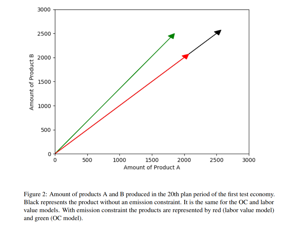
But if you now introduce an emission constraint and say we can’t overall emit more CO2, or more greenhouse gases, than a certain cap, then what happens in the labour value model – at least in some cases that I looked into – is that you simply produce less overall. So you don’t change the proportions. You don’t say we’re going to produce less meat because it’s environmentally destructive, but we’re going to keep producing as much of the veggie option or even more of the veggie option. No, instead, what you do is you keep the proportions one-to-one. You just produce less overall, because that’s all you can produce without violating the emissions constraint. But there’s no change in the proportions, because there’s no change in the in the calculated cost of producing these items.

Emissions aren’t factored into labour values. So meat doesn’t get a higher cost of production, just because you now want to limit the amount of emissions and it takes a lot of emissions to produce. So that’s not factored into the cost. And accordingly, it doesn’t factor into the mix of products being produced.

But what happens in my opportunity cost value model is that meat actually – when you introduce an emission constraint – gets a much higher opportunity cost. Because all those emission rights being used to produce meat could be used to produce a lot of other things. And that increases the cost of meat, and this then results in there being a lot less meat being produced. Because it has a higher cost and not as many people are willing to pay that high of a price, such that the cost and the prices are somehow balanced. So, you see actually not just a reduction in the overall production to meet the emission constraint. You see a drastic reduction in meat production, but a relative increase of the production of the veggie option, the environmentally friendly option.

[ATO] Yes, it’s very interesting. And I’m going to include pictures from the paper. Visually, this is represented as – you can think about this plan target as being a vector.

[PD] The plan target gives you gives you the direction of a vector. So, you have a product space. Because you just have two products, it’s two dimensional. That’s why I chose two products, it’s easier to them to understand. And the target tells you in which direction is that arrow going to be. Because it tells you the proportions at which products are being produced. And then the length of the vector tells you how much we are producing at these proportions.

And without emissions, basically, you get a one-to-one proportion. So the vector is at a 45 degree angle. And the length is as long as possible with available resources, not taking into account the emissions. You can produce as many emissions as you want, or as necessary to produce as much as is possible.

And so the in the labour value model, when you then introduce an emission constraint, what happens is the direction of the arrow remains the same, you simply decrease the length of the arrow. So, you will maintain the same proportions but produce less of all. While, in my model, you actually change the direction of the vector towards the environmentally friendly product. So you actually see a shift in the kinds of things being produced and not just the quantity of what has been produced.

[ATO] Yes, exactly. So what other results did you get?

[PD] This was the main thing that I was interested in. I also ran some tests to see what the computational complexity was. I used linear programming and my results were consistent with other tests of that Paul Cockshott did on the complexity of linear programming for these kinds of planning problems.

But the main thing that I was interested in was precisely this. How other factors than labour, in particular emission rates, affect the costs of producing items compared to labour values, and how that then affects the composition of products being produced. And the results were for the most part, consistent with my expectation; and I think demonstrate that opportunity costs are a more adequate measure of cost and that it really matters which one we choose, because it will lead to different a different mix of products being produced.

[ATO] Yes, the simulation is very interesting. Of course, it’s basically a proof of concept, because there’s a toy economy. But I think, yes, it does show that – like you were describing – there is a qualitative difference between the labour value model and the opportunity cost value model. In one you have the same plan target, the same product mix for the economy, and you’re just scaling that up and down. The opportunity cost model is more dynamic, in the sense that the mix can actually change.

Okay, so we’ve talked about the model, we’ve talked about the simulations. What work remains to be done, do you think?

[PD] There are a lot of simplifications in my simulation. And what could be done is to have a more refined version of it, which takes us to kind of other things which I haven’t taken into account.

For example, one major limitation of my simulation is that it doesn’t really consider economic growth and change in the capital stock. You don’t have a scenario where, for example, what you can produce in the second year depends on the machinery that you produced in the first year. So that’s currently not taking into account in my simulation.

There is literature on this. Paul Cockshott has written about multiyear plans where you get precisely this, what you produce in the second year depends on the machinery that’s available which can be also produced in the prior year, and built up, and so on. But there is, as far as I know, no model yet which tries to combine this these multiyear plans with consumer feedback. So you have the short term planning, where you don’t really see a change in the composition of capital goods, which is in response to consumer goods. That’s what I did. You have these multiyear plans where you do see a change in the composition of capital goods, and you can build up capital stock, and so on. But that wasn’t made responsive to consumer demand.

So, I think what should be done next is to have a model which does both, where you have constant changing capital stuff but the production specifically of consumer products, is also made responsive to consumer demand; and the proportions at which various products are being produced continually get adjusted, depending on consumer demand.

[ATO] And is that something that you think you’ll find yourself working on?

[PD] So at the moment, I’m not working on that yet. Maybe that’s something I’ll get the time to get to at some point.

At the moment, I’m working on some questions which are more related to philosophy. So I’m working on Marx’s concept of alienation and looking how that applies to a socialist society. Marx criticised capitalism because he thought that labour was alienated under capitalism. And then the question I asked myself is ‘well, isn’t labour still alienated under socialism? What’s different under socialism that suddenly people are not alienated, but are free in some sense?’. So that’s what I’m currently working on.

And the other thing I’m working on is I’m in active exchange with economists from the Austrian School of Economics, who have long criticised the feasibility of socialist planning. And we are discussing whether these cyber-socialist models – or sometimes they call them techno-socialist models – are an adequate response to this socialist calculation problem, which they think is a fundamental problem of socialism. So I’m engaged in active exchanges with them. There’s a special issue, it’s going to come out, I think, sometime later this year, or maybe next year, which will be an exchange along those lines.

And then I’m also working on a paper with political scientist Dan Greenwood where we really try to see where this debate is currently at. Which problems of socialism is the cybersocialist models, such as the ones we discussed, able to overcome and which problems maybe still remain?

[ATO] For the people watching, you’re saying that there’s work remaining to be done on integrating an opportunity cost model of central planning with consumer feedback with a multi-year investment planning model. And so if there’s somebody watching who thinks that they’re up to the task, that’s something to consider

We’ll leave it there. Thank you very much for joining me, again, Philip Dapprich, talking about introducing opportunity cost valuations and multiple production techniques into central planning. Because these are, these are two of the most fundamental issues, most fundamental criticisms, that can be made of central planning as a model. And so it’s very interesting to see the work that you’ve been doing. It’s very interesting and important on a general note.

In terms of this channel, I focus largely on post-capitalist futures. I think there are essentially three main categories, I think, of both capitalist features. The first is some variety of market socialism. The other is central planning. And then there’s economic planning, it’s in another way. So Participatory Economics is the best example. And what I’m interested in is in each of these models has been developed to its greatest extent. I think we all benefit from that. I’m not interested in just picking a horse, and following that. I certainly have opinions on what I think is good about each of these. I think that the work you’re doing is very important is what I’m trying to say.

[PD] Yes, thank you very much. And I agree that it’s important to consider different models. And obviously, I have I have a horse in this race. But I’m also always interested in engaging with alternative approaches. And I think there’s, for example, a serious debate to be had about what role of markets can or should play under socialism. Obviously, under certain circumstances, they can yield efficient outcomes. I think what I’m trying to show is that, I mean, we do use something like markets for consumer products, something vaguely resembling markets anyways. What I’m trying to show is that maybe you don’t need markets to determine an optimal plan. Maybe you can actually do it in another way as well. But even if that’s right, that doesn’t necessarily mean that it’s the best way. So, I think we need to look into other models as well and need to have these discussions. And yes, it’s good that people are working on other proposals.

[ATO] Okay. But it’s been great to talk about your proposal. And so thank you very much for joining me.

[PD] Yes, thank you so much. It was very pleasant discussion.

[ATO] Thank you for watching.

If you got anything from this video, then please press the Like button, consider Subscribing, and, if you really enjoyed it, then repeat every word at the top of your lungs like they did in Occupy Wall Street.

There’s a lot more to come. We’ll keep exploring better futures for humanity until we get there.

And as always, I want to read your thoughts in the Comments section below. This channel has a wonderful audience, and there are usually some very interesting comments under the video, so let’s continue that.

That’s all for now. Our democratic future lies After The Oligarchy.

References

Dapprich, Jan Philipp (2021). Optimal Planning with Consumer Feedback: A Simulation of a Socialist Economy.

Dapprich, Jan Philipp (2020). Rationality and Distribution in the Socialist Economy. PhD thesis.